1.1. Campo data and visualisation basics for point objects¶

1.1.1. Introduction & data set¶

In this exercise you will use the Campo Python module to execute static operations on fields and agents. You will use a data set of household locations and food outlets that also will be used in the spatio-temporal modelling exercises with Campo.

Campo is a model building framework for construction of field-agent based models, info is at https://campo.computationalgeography.org. You will have access to the capabilities of Campo through the Campo Python module. Under the hood, Campo uses several libraries. An important one is the LUE library for storing data containing both agents and fields. Information on LUE is at https://lue.computationalgeography.org. Note however that for the exercises below you will access LUE data always through Campo, so it is most important to understand Campo concepts.

Campo is still under development and in this exercise you will only use a subset of components of Campo as other components have not yet been documented and tested.

1.1.2. Phenomena, property sets and point objects¶

Open the template file static_model.py in your text editor and inspect it. The script imports the necessary Python modules and creates the static model class FoodEnvironment. You will add your model processes, i.e. operations on fields or agents, to the initial section of the model script. Processes stated in this section will be executed once when running the model.

We will model propensity for healthy food of households and use household locations and shop locations in the municipality of Utrecht, the Netherlands, for our model. The locations of stores and household are stored in two separate text files that we will use later on.

To add phenomena to a model you first need to initialize a model data object. Replace pass from the initial method and replace it by the following:

foodenv = campo.Campo()

Execute the script, it shouldn’t print anything. The foodenv object will provide access to the methods for constructing agents, and eventually arrange the storage to the LUE dataset on disk.

A particular ‘thing’ that is represented by your model is represented by a ‘phenomenon’ in Campo. A phenomenon contains multiple agents or individuals, referred to as ‘objects’ in Campo. Examples of a phenomenon are trees, cars, catchments. Here we will create the phenomenon foodstores. To create a phenomenon, the add_phenomenon function is used. Add the phenomenon foodstores to the foodenv data object by typing the following statement in the initial part of the script:

foodstores = foodenv.add_phenomenon("foodstores")

Execute the script, again it shouldn’t print anything.

Each object (agent, individual) in a phenomenon can have multiple properties attached to it, for instance color, weight, biomass. Properties can exist only at one location (x,y), for instance at the front door of a foodstore. These are so called point properties. Alternatively, properties can also exist in a spatial extent defined by a bounding box, which are called field properties. We will first focus on point properties. All point properties within a phenomenon are grouped together in a so called ‘property set’.

Open the file foodstores_frontdoor.csv and have a look at its contents. Each row contains the (x,y) coordinates of a foodstore. Close the file without changing its content. We will create objects inside foodstores by reading from this file. Add the following statement:

foodstores.add_property_set("frontdoor", "foodstores_frontdoor.csv")

The first arguments assigns the name of the property set that is created and the second the input file name. Inside the foodstores phenomenon, Campo will create a number of objects equal to the number of lines in the input csv file, and a property set named frontdoor with a point location for each object (at the location of the coordinate given in the csv file).

1.1.3. Point properties¶

So far you have only defined the domain of the data set: the number of objects, and a property set (frontdoor) defining a location for each object. It is now time to add actual property values to this property set.

You can add properties by just using the dot notation on property sets and initialize them directly, e.g. setting the four digit postal_code to 1234 can be done by:

foodstores.frontdoor.postal_code = 1234

This will assign the value 1234 to the postal code property value of each object.

You can also assign random values drawn from a uniform distribution as follows:

foodstores.frontdoor.lower = -0.5
foodstores.frontdoor.upper = 0.5
foodstores.frontdoor.x_initial = campo.uniform(foodstores.frontdoor.lower, foodstores.frontdoor.upper)

The first two statements set the lower and the upper bounds of the uniform distribution. The third statement draws a random value between these bounds for each object and assigns it to the property x_initial. This property refers to the quality of food (also, propensity) offered by the foodstore. Below zero implies unhealthy while above zero implies healthy food. You will in the spatio-temporal modelling exercise how this is used to model dietary habits over the city.

Question: What is a uniform distribution? Why would one use in certain cases a uniform distribution instead of the often used Gaussian distribution?

1.1.4. Writing data to disk and visualisation of point properties¶

All information in the LUE data set and properties you created so far exist only in memory. To store those to disk you need to perform a few additional steps at the end of your initial section. First create a LUE data set with the name food_environment.lue:

foodenv.create_dataset("food_environment.lue")

All phenomena, property sets and properties can then be stored in the LUE dataset by adding at the end of your initial section.

foodenv.write()

Run the script again and check if the lue file is stored on your hard disk. It should be in the same folder as your model.

You can open the lue file with the script plot_point_objects.py. Inspect it. The first function reads the data set from disk assigning it to dataset. The second function campo.dataframe.select can be used to read data from the lue dataset storing it in a standard Python data structure. Its first argument defines from which phenomenon data is read (here, foodstores), the second argument defines a list of strings defining which properties one would like to read, here x_initial. Add two lines at the bottom:

print(dataframe)
print(type(dataframe))

You will notice that for point objects, dataframe returned by the function is a dictionary showing the objects per row and property values per column.

For plotting you may want to export the contents of dataframe to a .csv file. You can do this by adding at the bottom:

campo.to_csv(dataframe, 'foodstores.csv')

Run the script and inspect the contents of the csv file. It contains the (x,y) coordinates of each object with the x_initial value added. Of course you can use the csv file to plot the data.

Alternatively you can export data to a GeoPackage file (GPKG) and then visualise in a GIS. To do so, add the following line to plot_point_objects.py:

campo.to_gpkg(dataframe, 'foodstores.gpkg', 'EPSG:28992')

It creates foodstores.gpkg which can for instance be displayed with QGIS. If you have QGIS installed in your Conda environment you can simply type:

qgis data/roads.gpkg foodstores.gpkg

It will open QGIS with the foodstore data and a roads layer for context. If QGIS is not in your Conda environment start it up like normal and then open the same files as layers by dragging them from the Browser window into the Layers window. In QGIS you can inspect property values with the Identify Features pointer (click on top of window on the button with the ‘i’ symbol). Or visualise them: right-click on ‘foodstores’ in the Layer window, select Properties, select Symbology, click on Symbol and change to Graduated, select for Value the property you want to show, for instance x_initial, click on Classify, click on OK. A filled colour is used to represent the value of the Property. Alternatively, you can select in the Graduated page also for Method: Size which shows the shops sized according to the Property value. Do not forget to click ‘Classify’. For additional explanation refer to https://docs.qgis.org/2.18/en/docs/user_manual/working_with_vector/vector_properties.html.

1.2. Operations on point properties within a property set¶

1.2.1. Local operations¶

Local operations on point properties simply update the property values by using arithmic operations, comparisons, etc. Open the script static_point_operations.py which is the script containing everything that you added in the exercises above. You will create now a propensity value foodstores.frontdoor.x_value by incrementing the initial value x_initial with a small random number. Add the following code to the script, just above the create_dataset function and run the script.

foodstores.frontdoor.lower_inc = 0.0
foodstores.frontdoor.upper_inc = 0.1
foodstores.frontdoor.increment = campo.uniform(foodstores.frontdoor.lower_inc, foodstores.frontdoor.upper_inc)

foodstores.frontdoor.x_value = foodstores.frontdoor.x_initial + foodstores.frontdoor.increment
foodstores.frontdoor.threshold = 0.0
foodstores.frontdoor.healthy = foodstores.frontdoor.x_value <= foodstores.frontdoor.threshold

Modify the plot_point_objects.py script to inspect the result and check the calculations.

1.3. Campo data and visualisation basics for field objects¶

1.3.1. Field properties and operations on field properties within a property set¶

In Campo, a phenomenon can include multiple property sets, where property sets are different regarding the spatial domain of the data. In the previous example you created a frontdoor property set inside foodstores. This had a point domain: each object was linked to a single location, the front door. Now we will add a second property set to the foodstores to simulate the spatial processes in the surrounding of each store. This is referred to as a field-agent.

Question: Give two other examples of the use of field-agents in spatial or spatio-temporal simulation.

Open the file foodstores_surrounding.csv. Each line gives the four corners of a bounding box surrounding a foodstore. The last two values give the number of rows and columns. In general, the spatial extents can be for all agents of the same size (e.g. fixed sized neighbourhoods), or the extents can differ between agents (e.g. different catchments). In our example we will consider the surrounding of the food stores with constant neighbourhood sizes per agent.

Open static_model_fields.py, it contains the main part used in the previous exercises.

In general, field agents are added comparably to the point agents with the add_property_set function. Add this function at the bottom of the script, reading foodstores_surrounding.csv and creating a new property set surrounding. Run the script to check if all is fine.

Now let’s do the same uniform operation to create a field property inside the surrounding property set. Add this in the initial (at the bottom, but above the write statement):

foodstores.surrounding.lower = 3
foodstores.surrounding.upper = 12
foodstores.surrounding.c = campo.uniform(foodstores.surrounding.lower, foodstores.surrounding.upper)

Again run the script. In the next section you will inspect the result.

1.3.2. Writing data to disk and visualisation of field properties¶

To visualise field properties you can use plot_field_objects.py. Open the file and inspect it. Just like with the point properties, it opens the data set, and selects a property name, this time c. This is the property created in the previous section, a field property. The to_tiff function converts the field property value (here, c) for each object to a separate geotiff file, with file names c_1.tiff, c_2.tiff, etc. Run the script - it will print the content of c. Then, open some of the geotiff files (not all, as it may be too much for your computer) with a GIS, for instance QGIS. Again, if you have QGIS installed in your Conda environment, you could simply type the following command, which will open a subet of the files:

qgis data/roads.gpkg c_*0.tiff foodstores.gpkg

Just like with point objects, you can inspect cell values by selecting Identify Features and clicking on the map. Note that only values from an active geotiff file are plotted, to activate a layer, click on it (not uncheck/check as this determines whether the layer is displayed) in the Layers window. You may want to drag them all to a layer group which you can create in the Layers panel; this will allow you to check or uncheck them all (right-click on the layer group after dragging all geotiffs to the group). Refer to the QGIS manual for details https://docs.qgis.org/3.16/en/docs/user_manual/introduction/general_tools.html.

1.4. Operations on field properties within a property set¶

1.4.1. Distance calculation¶

With a two-dimensional raster-based spatial domain we particularly can execute spatial operations on the agents of a property set. You can, for example, calculate for each food store the distances to other foodstores within their spatial surrounding. This can be done with the spread(start_locations, initial_friction, friction) operation calculating for each cell the shortest distance to non zero cells.

First, you need to create a raster with locations of food stores in a surrounding. Use the feature_to_raster operation:

foodstores.surrounding.start_locations = campo.feature_to_raster(foodstores.surrounding, foodstores.frontdoor)

First input argument to the operation is the field property set holding the spatial surrounding of each food store, second argument are the front door locations of all the food stores in the modelling area. Return value of the operation is a raster with values of 1 for cells with corresponding food store locations and 0 otherwise. Note that this is a specific operation that has input arguments from two different property sets, surrounding and frontdoor.

Add the operation to the static_model_fields.py script. Run the script and visualise the output using plot_field_objects.py used in the previous section.

Now add the spread operation (syntax given above). You also need to create properties for the other two arguments of the spread operation, the initial friction distance (use the value 0) and the friction (use the value 1). Using these two values you calculate the absolute distances (in metres). Add the operation, run the script, and have a look at the result using plot_field_objects.py.

When you have this running, try creating a zone within 200 m from each food outlet

foodstores.surrounding.area = foodstores.surrounding.distance <= 200

Run the script and once more look at the result using plot_field_objects.py.

1.5. Operations between property sets: combining different phenomena and property sets¶

So far we mainly did calculations on property values within a certain property set of one and the same phenomenon. In many models however calculations are done between phenomena. An example is the focal_agents function which is similar to a focal, window, or convolution operation, but now applied on agents. The syntax is:

a.points.y = campo.focal_agents(a.points, a.fields.w, b.points.x)

It has inputs from two phenomena, a and b. The input b.points.x is a property belonging to the point property set b.points. For each object in b, x has a certain point value. The input a.fields.w is a property belonging to the field property set a.fields. For each object in a, property b is a raster where each raster cell contains a value. The input a.points merely sets the property set to return. The result is a.points.y, which is a property set in the point domain a.points. The function calculates for each object in a, the average value of all property values in the other phenomenon (b.points.x). The average value is a weighted average, where the weights are the values from a.fields.w at the location of each object in b.points. In an equation:

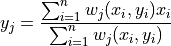
$\ y_j = \frac{\sum_{i=1}^{n} w_{j} (x_i,y_i) x_i }{\sum_{i=1}^{n} w_{j} (x_i,y_i)}$

The equation shows the calculation of the return value $y_j$ , which is a.points.y for the $j$ th object in a. It is used for each object $j$ in a. It uses:

$x_i$ , the value of the $i$ th object of b.points.x, and
$w_j(x_i,y_i)$ , the value of a.fields.w for the $j$ th object in a at the location $(x_i, y_i)$ of $i$ th object of b.points.

To illustrate the use of focal_agents, consider the case where we are modelling the healthiness of food offered for sale at foodstores. The stores will adjust their product range to the dietary habits of their customers, that is, the households in the surroundings of a store. This mechanism can be modelled with the focal_agents operation. Open the script static_two_phen.py. It defines two phenomena, foodstores, and households. The households contain a property households.frontdoor.x, which is the households` propensity for eating healthy food. Here, we assign a random value between -2.0 and 2.0 to each household (we will expand upon this in the temporal modelling exercises!).

The foodstores contain two properties important for the calculation. The property foodstores.surrounding.weight gives for each store the weight in its surroundings (field-property). Be sure to understand how this weight is calculated (using the spread and where functions). The property foodstores.frontdoor.y is the healthiness of the food offered by the store, which is the average of the surrounding households, but weighted by foodstores.surrounding.weight.

Run the script and then inspect plot_two_phen.py which converts the outputs to files that you can view with QGIS, like in the previous exercises.

Open foodstores.gpkg, households.gpkg, as well as area_143.tiff and weight_143.tiff with QGIS. The two tiff files contain foodstores.surrounding.area and foodstores.surrounding.weight properties for object id 143 in the phenomenon foodstores. Check the calculation of foodstores.frontdoor.y by inspecting the y-value in foodstores.gpkg for object id 143. Note that it is a weighted sum of the x-values of households.gpkg, weighted by weight_143.tiff.

As you will have noticed the script assumes that a shop attracts customers up to a distance of 250 m away from the shop, this is defined in the operation calculating foodstores.surrounding.area. Change this value to 500 m and rerun the script. Again display the output for object id 143 and compare the results.

Question: What is approximately the range of values in the propensity of the foodstores? Compare this with the range in the propensity of the households. What is causing the observed difference?

Question: What is the effect of the size of the neigbhourhood, for instance 250 or 500 m, on the resulting range in propensity values of the foodstores? Explain your answer.