2.1. Point agents¶

In the spatio-temporal modelling exercises we will stepwise build a spatial model that simulates how the propensity for a healthy diet of households changes over time, in interaction with the healthiness of food offered at food stores. But we will first neglect the effect of the food stores. The propensity for healthy food of a household can be simulated with the following differential equation:

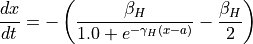
$\frac{dx}{dt} = -\left( \frac{\beta_{H}}{1.0 + e^{-\gamma_{H} (x - a)}} - \frac{\beta_{H}}{2} \right)$

In the equation, $x$ is the propensity for healthy food of a household. The equation gives how it changes over time, as a function of the parameters $beta_{H}$ , $gamma_{H}$ , and a. The equation looks complicated but it is a simple curve. To plot the curve, open, inspect, and run equations.py. It creates equations.pdf. Neglect the second and third row of the pdf. The first plot in the first row is a plot of the equation above. The x-axis is $x$ , the propensity of the household; the y-axis is $dx/dt$ , the rate of change of the propensity over time. For propensity values with a positive rate of change, the propensity will increase over time, while with negative rates, it will decrease over time.

If you inspect the curve, you can see that the propensity will always tend to a value of zero in this case. This is a so called stable state. It is equal to the value of the parameter a, which we call the default propensity of the households. We assume for now it is the same for all households, zero. Propensities above zero refer to healthy food, while propensities below zero refer to unhealthy food. The idea here is that households will have a default value of the healthiness of their diet, which is set by the properties of the houshold itself (e.g. income, genes, etc). By external forcing, the propensity may change, but it will tend back to the default value. At least if we use only this equation!

Now it is time to run a spatio-temporal model that uses the equation to calculate how the propensity changes over time. Inspect households.py. It uses the same dataset from the static modelling exercises, but now defining all parameters from the equation above, in the initial section. In the dynamic section, then, the propensity, self.hh.fd.x is updated for each timestep, using the equation given above. The time step duration is 3 months. We assume that at the start of the run, each household has a random propensity between -2 and 2.

Run the model. Inspect plot_households.py, which can be used to visualise the outputs. Just like in the static modelling exercises, it converts the output to gpkg files, but now for each timestep. They are written as households_1.gpkg, households_2.gpkg, etc. The second part of the script converts the propensity values x to a .csv file, which is then converted to a pdf. Each line in the pdf shows the change of the propensity over time of one household.

Run plot_households.py and open the households_x.pdf file. Also, open the gpkg files using QGIS. You could open them all as well as the road network from the folder data. In QGIS, visualise the values just like in the static modelling exercises. It is important to use the same Styles for each layer (time step) to enable comparison between timesteps. To do so, set the style for the first time step, households_1: right-click on the layer, select Properties, select Symbology, click on Single symbol and change it to graduated. Then, select the Value to be plotted (x), use Method: color, click on Classify. Click on OK. The color of the symbols now represents the propensity. Now, you can copy the settings to the other layers: right-click on the households_1 layer in the Layer panel and select Styles, Copy Style, All Style Categories. Now you can paste the copied style to another layer, by right clicking on another layer. Do it for multiple layers. By selecting or deselecting layers you can show or hide them and inspect how values change over time.

Question: How does the value of the propensity change over time? What are the values at the last time step?

2.2. Field agents used for input in temporal model¶

Of course the dietary habits of households is not only influenced by internal household processes (represented in the previous section) but also by their influences from outside. For instance dietary habits in their social network or the healthiness of food offered in stores. If the food offered at stores is more healthy than a households` default propensity (represented by the parameter $a$ ) the actual propensity of the household will tend to be higher due to the influence of the food in the stores. This effect is modelled by our second model, which adds a second term, the effect of the healthiness of food offered at the store where the household is shopping. We refer to this food in the store as ‘propensity’ as well, represented by the symbol $y$ in the equation below:

$\frac{dx}{dt} = -\left( \frac{\beta_{H}}{1.0 + e^{-\gamma_{H} (x - a)}} - \frac{\beta_{H}}{2} \right) + \left( \frac{\beta_{S}}{1.0 + e^{-\gamma_{S} (y - a)}} - \frac{\beta_{S}}{2} \right)$

To keep things simple, we use the same shape for the curve of the second term, however with a minus added and we will use slightly different parameter values. To inspect the curve of the second term, run equations.py and open the second pdf created by the script, equation_food_store_effect.pdf. Note that the x-axis gives propensity values of the food offered at a nearby store, the y-axis gives the corresponding rate of change in the propensity of the household (the outcome of the second term above). For now, we will assume that all stores offer food with a propensity of 0.2. As shown by the dashed orange line, this results in a rate of change (y-axis) of about 1.19 (year-1). So the value of the second term for our example is 1.19.

To understand the values of the terms in the equation above, inspect equations.pdf again, in particular the second row. The first curve in the second row gives the value of the first term in the equation above, the so-called household effect. The second curve, then, gives the effect of the food outlet. For all household propensities (x-axis), the contribution to the rate of change is 1.19. The total rate of change, now, is the sum of the two curves, shown in the right plot (centre row). The position where the line crosses the x-axis is the equilibrium propensity of the households. As you can see, this is somewhat above 0.0, as a result of the influence of the food stores.

How does this influence the spatial pattern of household propensity? One would like to know how spatial patterns of propensity change driven by a certain spatial pattern of propensities of food stores. This can be evaluated with households_foodstores.py, defining from top to bottom:

Two terms of the differential equation above.
No changes have been made to the part of the script defining the starting values for the households.
The foodstores phenomenon. As we do not have observed propensities available now, we generate food store propensities self.fs.hd.y that are either 0.0 (70% of them) or 0.2. The stores with 0.2 are randomly selected.
The average of the propensity of food stores in the neighbourhood of each household, self.hh.fd.y. It is calculated using the focal operation just like we did in the static modelling exercises. The property self.hh.fd.y represents $y$ in the equation above.
The differential equation with the food store propensity effect added (dynamic section).

Run the script. Inspect plot_households_foodstores.py used for creating the output visualisations. Run the script and inspect the results.

Question: What is the highest value of the household propensity in the area at the end of the model run? Does it correspond with what you would expect from the value of the differential equation plot in equations.pdf, centre row, right plot?

2.3. Field agents in a temporal simulation¶

As a next step we will evaluate how households and food stores interact, leading to the emergence of spatial patterns in propensity. In the previous exercise we simulated the influence of the healthiness of food at foodstores on the healthiness of food consumed by households. We fixed the propensity of the foodstores. In reality, of course, food stores adjust the products offered to the products consumed. In this exercise we incorporate this mechanism by one simple addition to the model: for each time step the propensity of food stores is assumed to be equal to that of the propensity of the households in their surroundings. So, both food store propensity and household propensity are updated as a function of their surroundings, for each time step.

This concept leads to a full coupling of the households and foodstores. This can be understood with the help of the plots in the bottom row of equations.pdf. The first plot is still the same, it refers to the first term of the differential equation. As we assume now that food store propensity is equal to household propensity, the second plot changes. Instead of a fixed rate of change like in the previous exercise (centre row), the curve now follows the second term of the differential equation, where the rate of change changes with the propensity of the households (which is equal to that of the food stores in their surrounding). The total effect in the third column shows that two stable equilibria appear, one for propensities around -2 and another one for propensities around 2.

This approach has been coded in households_foodstores_inter.py. The main differences with the previous script are:

Instead of fixing the food store propensity self.fs.fd.y it is now calculated as the average household propensity in the surroundings, in the dynamic section.
As food store propensities change over time, self.hh.fd.y is now calculated for each time step as the average of the food store propensities in the surroundings of a household.

Run the model. It will take some time as the focal_agents operations now need to be done for each time step. Inspect plot_households_foodstores_inter.py to see what outputs are converted and run the script. View the output pdf files as well as the gpkg files with QGIS.

Question: What is the spatial pattern in the household propensities at the start, halfway, and at the end of the run? Explain the mechanisms that determine the spatial pattern and how it changes over time.